Trying my first JavaFX Program

So, I've looked up some websites on JavaFX as I wanted to quickly throw something nice together for drawing Geometry.

You can find my little tool on the GitHub¹.

It works fine for what I needed. I wanted to be able to quickly show the difference between geometries.

The tool uses locationtech for geometry stuff, and javafx for display stuff.

It accepts WKT representations of geometry. Currently, these do not provide any coordinate systems, so you're unlucky there.

I did get the error:

Error: JavaFX runtime components are missing, and are required to run this application

But I changed my app to pull JavaFX from Maven Central and that seems to fixed the issues. JavaFX is no longer included in any JDK.

References

[1] GitHub.com - geoviewer

https://github.com/maartenl/geoviewer

JavaFX - Getting Started with JavaFX

https://openjfx.io/openjfx-docs/#maven

developer.com - Using Graphics in JavaFX

https://www.developer.com/open-source/using-graphics-in-javafx/

JavaFX - Main website

https://openjfx.io/

Using SQL Developer to visualise Geometry data

I was looking to see if shapes were incorporated inside other shapes.

I could have let the database check this, but sometimes it is very insightful to have a visual representation.

It turns out, SQL Developer facilitates this.

If you select a geometry field in your table, and right click and select [Display geometry shape], you'll get a nice little window indicating the shape.

Sometimes this is greyed out. The solution for this is to click on [Edit] in the menu above, and select [Map View]. This will "initialize" stuff, and then it's no longer greyed out.

Map View

The map view is very convenient, if you wish to show multiple shapes and how they interact.

To get started, select under "View", "Map view" and you are presented with a new subwindow.

Pressting the "New" button in the Map View window, you can just enter a query that returns a geometry, give it a name, proper colouring, and you're good to go.

In the example above, there's two queries, one for a point and one for a shape. The Map View displays them both, and you can even deactive one or the other in the table on the right.

Very convenient in my work, I say.

References

[1] ThatJeffSmith - Visualize Spatial Data with SQL Developer

https://www.thatjeffsmith.com/archive/2011/12/visualize-spatial-data-with-sql-developer/

Spatial Information in an Oracle Database

SDO_GEOMETRY

This is here for me to remember how much magic is used in inserting spatial (geometry) information into an Oracle database¹.

CREATE TYPE sdo_geometry AS OBJECT (
SDO_GTYPE NUMBER,
SDO_SRID NUMBER,
SDO_POINT SDO_POINT_TYPE,
SDO_ELEM_INFO SDO_ELEM_INFO_ARRAY,
SDO_ORDINATES SDO_ORDINATE_ARRAY);

A point geometry:

MDSYS.SDO_GEOMETRY(
    2001, -- 2-dimensional (2), non-linear referencing geometry or default (0), point (01)
    28992, -- Amersfoort / RD New
    NULL, 
    MDSYS.SDO_ELEM_INFO_ARRAY(1, 1, 1),
    MDSYS.SDO_ORDINATE_ARRAY(81431.756, 455218.921))

A polygon geometry:

MDSYS.SDO_GEOMETRY(
    2003, -- 2-dimensional (2), non-linear referencing geometry or default (0), polygon (03)
    28992, -- Amersfoort / RD New
    NULL,
    MDSYS.SDO_ELEM_INFO_ARRAY(1,1003,1), -- first coordinate (1), exterior (1003), polygon (1)
    MDSYS.SDO_ORDINATE_ARRAY(
        -1041172.16,1407540.16,
        -958596.8,-591471.68,
        1363835.2,-625878.08,
        1319106.88,1428184,
        -1041172.16,1407540.16) -- coordinates
)

A multipolygon geometry:

MDSYS.SDO_GEOMETRY(
    2007, -- 2-dimensional (2), non-linear referencing geometry or default (0), MULTIPOLYGON or MULTISURFACE (07)
    28992, -- Amersfoort / RD New
    NULL, 
    MDSYS.SDO_ELEM_INFO_ARRAY(1, 1003, 1, 11, 2003, 1), 
    MDSYS.SDO_ORDINATE_ARRAY(42, 78, 41, 85, 46, 82.7, 45, 79, 42, 78, 43.5, 72.5, 52.5, 72.5, 54.5, 79.5, 79, 60, 93, 46, 53, 32, 54, 25, 49, 22, 45, 17, 41, 16, 37, 23, 33, 24, 25, 20, 33, 46, 39, 53, 43.5, 72.5))

The only thing that makes sense among all the magic numbers are the coordinates. The last coordinate is the same as the first coordinate to close the polygon.

I since have found some more information after some digging regarding the SDO_ELEM_INFO.

It's an array of triplets, where a triplet consists of:

SDO_STARTING_OFFSET

offset within the coordinates array, the first triplet usually has "1" as being the first coordinate in the coordinate array

SDO_ETYPE

type of element

SDO_INTERPRETATION

depends on if SDO_ETYPE is a compound element

I found more information in [2].

WKT - Well-known text representation of geometry

"POLYGON ((194232.738 467652.498, 194232.774322728 467652.19885542, 194232.881179968 467651.917096035, 194232.738 467652.498))"

"POINT (31256.383 393077.6)"

"MULTIPOLYGON(((42 78, 41 85, 46 82.7, 45 79, 42 78),(43.5 72.5, 52.5 72.5, 54.5 79.5, 79 60, 93 46, 53 32, 54 25, 49 22, 45 17, 41 16, 37 23, 33 24, 25 20, 33 46, 39 53, 43.5 72.5)))"

It's possible to create SDO_GEOMETRY in PL/SQL based on WKT strings.

Like so:

SELECT SDO_GEOMETRY('MULTIPOLYGON(((42 78, 41 85, 46 82.7, 45 79, 42 78),(43.5 72.5, 52.5 72.5, 54.5 79.5, 79 60, 93 46, 53 32, 54 25, 49 22, 45 17, 41 16, 37 23, 33 24, 25 20, 33 46, 39 53, 43.5 72.5)))') FROM DUAL;

Convenient if you want to do something quick, but you cannot provide additional information regarding the dimensions, and coordinate system, etc.

Let me rephrase that sentence. It means your resulting geometrie has NO SRID, and you'll get in trouble using it in geometry queries! This is not a joke!

The reverse (if you want to find out the geometrie in WKT format, basically because it reads easier) is of course also possible, like so:

SELECT SDO_UTIL.TO_WKTGEOMETRY(geometry) FROM buildinggeo;

Geometry Functions

So I was playing around with ConvexHull, ConcaveHull and ConcaveHull-Boundary functions.

I took the MultiPolygon in the paragraph above as an example.

SELECT SDO_GEOM.SDO_CONVEXHULL(MDSYS.SDO_GEOMETRY(
2007, -- 2-dimensional (2), non-linear referencing geometry or default (0), multipolygon (07)
28992, -- Amersfoort / RD New
NULL,
MDSYS.SDO_ELEM_INFO_ARRAY(1,1003,1,11,2003,1), -- first coordinate (1), Simple polygon whose vertices are connected by straight line segments (1003,1), 11th coordinate (11), Simple polygon whose vertices are connected by straight line segments (1003,1)
MDSYS.SDO_ORDINATE_ARRAY(42, 78, 41, 85, 46, 82.7, 45, 79, 42, 78,
43.5, 72.5, 52.5, 72.5, 54.5, 79.5, 79, 60, 93, 46, 53, 32, 54, 25, 49, 22, 45, 17, 41, 16, 37, 23, 33, 24, 25, 20, 33, 46, 39, 53, 43.5, 72.5) -- coordinates
), 1)
FROM dual;
-- creates MDSYS.SDO_GEOMETRY(2003, 28992, NULL, MDSYS.SDO_ELEM_INFO_ARRAY(1, 1003, 1), MDSYS.SDO_ORDINATE_ARRAY(41, 16, 45, 17, 93, 46, 79, 60, 54.5, 79.5, 41, 85, 25, 20, 41, 16))

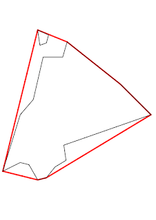
SELECT SDO_GEOM.SDO_CONCAVEHULL(MDSYS.SDO_GEOMETRY(
2007, -- 2-dimensional (2), non-linear referencing geometry or default (0), multipolygon (07)
28992, -- Amersfoort / RD New
NULL,
MDSYS.SDO_ELEM_INFO_ARRAY(1,1003,1,11,2003,1), -- first coordinate (1), Simple polygon whose vertices are connected by straight line segments (1003,1), 11th coordinate (11), Simple polygon whose vertices are connected by straight line segments (1003,1)
MDSYS.SDO_ORDINATE_ARRAY(42, 78, 41, 85, 46, 82.7, 45, 79, 42, 78,
43.5, 72.5, 52.5, 72.5, 54.5, 79.5, 79, 60, 93, 46, 53, 32, 54, 25, 49, 22, 45, 17, 41, 16, 37, 23, 33, 24, 25, 20, 33, 46, 39, 53, 43.5, 72.5) -- coordinates
), 0.1)
FROM dual;
-- creates MDSYS.SDO_GEOMETRY(2003, 28992, NULL, MDSYS.SDO_ELEM_INFO_ARRAY(1, 1003, 1), MDSYS.SDO_ORDINATE_ARRAY(41, 85, 42, 78, 43.5, 72.5, 39, 53, 33, 46, 25, 20, 41, 16, 45, 17, 54, 25, 53, 32, 93, 46, 79, 60, 54.5, 79.5, 46, 82.7, 41, 85))

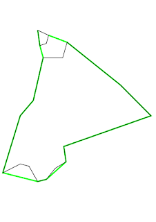
SELECT SDO_GEOM.SDO_CONCAVEHULL_BOUNDARY(MDSYS.SDO_GEOMETRY(
2007, -- 2-dimensional (2), non-linear referencing geometry or default (0), multipolygon (07)
28992, -- Amersfoort / RD New
NULL,
MDSYS.SDO_ELEM_INFO_ARRAY(1,1003,1,11,2003,1), -- first coordinate (1), Simple polygon whose vertices are connected by straight line segments (1003,1), 11th coordinate (11), Simple polygon whose vertices are connected by straight line segments (1003,1)
MDSYS.SDO_ORDINATE_ARRAY(42, 78, 41, 85, 46, 82.7, 45, 79, 42, 78,
43.5, 72.5, 52.5, 72.5, 54.5, 79.5, 79, 60, 93, 46, 53, 32, 54, 25, 49, 22, 45, 17, 41, 16, 37, 23, 33, 24, 25, 20, 33, 46, 39, 53, 43.5, 72.5) -- coordinates
), 0.1, 0.01)
FROM dual;
-- creates MDSYS.SDO_GEOMETRY(2003, 28992, NULL, MDSYS.SDO_ELEM_INFO_ARRAY(1, 1003, 1), MDSYS.SDO_ORDINATE_ARRAY(41, 85, 33, 46, 25, 20, 41, 16, 45, 17, 54, 25, 53, 32, 93, 46, 79, 60, 54.5, 79.5, 41, 85))

I will expand on this blog post, as my knowledge in this area is expanded.

References

[1] Spatial and Graph Developer's Guide - 2.2 SDO_GEOMETRY Object Type

https://docs.oracle.com/database/121/SPATL/sdo_geometry-object-type.htm#SPATL489

[2] Spatial and Graph Developer's Guide - 2.2.4 SDO_ELEM_INFO

https://docs.oracle.com/database/121/SPATL/sdo_geometry-object-type.htm#SPATL494

Spatial and Graph Developer's Guide - 2.1 Simple Example: Inserting, Indexing, and Querying Spatial Data

https://docs.oracle.com/database/121/SPATL/simple-example-inserting-indexing-and-querying-spatial-data.htm#SPATL486

Sum of 1 to 100

Back in school, during Math, one of the arithmetic examples that spoke the most to me about how Powerful Math can be, was the explanation for the adding up of the first one hundred numbers.

The short explanation

When you have a nice distribution of numbers like 1 to 100, it is obvious that the average is right down the middle, which is 50½. And given the fact that we have 100 numbers, the solution becomes obvious.

Okay, so for some people that explanation might have been a bit too short.

The Long Explanation

Determining the average of a series of numbers, \(x_{1}, x_{2}, x_{3}, ... x_{n-1}, x_{n}\) is done by summing them all, and then dividing by the amount of numbers you have.
\[x_{avg} = {\displaystyle\sum_{i=1}^{n} x_i \over n}\]
Therefore, it follows that the sum, i.e. the thing we wish to know, is obviously:
\[{\displaystyle\sum_{i=1}^{n} x_i} = n * x_{avg}\]
For the first 100 numbers, this gives:
\[{\displaystyle\sum_{i=1}^{100} x_i} = 100 * 50{1 \over 2} = 5050\]

The Staircase

Of course, most explanations use a bit more imagination to make things clear².

Think of the problem as a staircase, with steps reaching from 1 to 100. To make things a bit more simple, and to save my having to draw 100 steps, let's try it with 10 first. With 100 steps the principles are the same.

The interesting part here, is that we can pair different numbers. We will add the numbers at the outside of the figure above, 1 and 10. This gives 11. Next the following outside numbers 2 and 9, also gives 11. In a figure, this would look as follows:

Hence, the answer is the surface of the square, \(5 * 11 = 55\).

Triangles

Obviously the surface area of the square is equal to the surface area of the staircase. If you look at the staircase, you might see a triangle. The surface of the triangle is half the surface of the square containing the triangle (actually containing the two triangles, forming the square).

So you could compute the surface of the staircase also by computing the surface of the square and dividing by two. As it's not a perfect triangle, we need to do some cutting. In geometry, this would look something like the following:

Anecdote

The Anecdote that everybody knows or has heard relates that Carl Friedrich Gauss³, a German mathematician who contributed significantly to many fields, solved this problem in primary school.

References

[1] LaTeX Mathematics

http://en.wikibooks.org/wiki/LaTeX/Mathematics

[2] What is the sum of the first 100 whole numbers?

http://mathcentral.uregina.ca/QQ/database/QQ.02.06/jo1.html

[3] Wikipedia - Carl Friedrich Gauss

http://en.wikipedia.org/wiki/Carl_Friedrich_Gauss